Introduction Of Ms Excel
Excel 2013 is a spreadsheet program that allows you to store, organize, and analyze information. Excel is a powerful spreadsheet application that is perfect for maintaining long lists of data, budgets, sales figures and other data. Excel is in its most basic form, a very fancy calculator.
While you may believe Excel is only used by certain people to process complicated data, anyone can learn how to take advantage of the program’s powerful features. Whether you’re keeping a budget, or creating an invoice, Excel makes it easy to work with different types of data.
The three most common general uses for spreadsheet software are to create budgets, produce graphs and charts, and for storing and sorting data. Spreadsheet software is used to forecast future performance, calculate tax.
Spreadsheets will provide you with the values arranged in rows and columns that can be changed mathematically using both basic and complex arithmetic operations.
Getting to know Excel 2013
Excel 2013 is similar to Excel 2010. If you’ve previously used Excel 2010, Excel 2013 should feel familiar. If you are new to Excel or have more experience with older versions, you should first take some time to become familiar with the Excel 2013 interface.
When you open Excel 2013 for the first time, the Excel Start Screen will appear. From here, you’ll be able to create a new workbook, choose a template, and access your recently edited workbooks.
To create a new blank workbook:
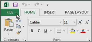
- Select the File tab. backstage view will appear.
- Select New, then click Blank workbook.
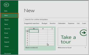
- A new blank workbook will appear.
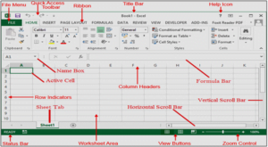
Understanding The Ribbon:-
The ribbon provides shortcuts to commands in Excel. A command is an action that the user performs. An example of a command is creating a new document, printing a documenting, etc.
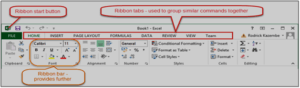
Ribbon start button – It is used to access commands i.e. creating new documents, saving existing work, printing, accessing the options for customizing Excel, etc.
Ribbon tabs – The tabs are used to group similar commands together. The home tab is used for basic commands such as formatting the data to make it more presentable, sorting and finding specific data within the spreadsheet.
Ribbon bar – The bars are used to group similar commands together. As an example, the Alignment ribbon bar is used to group all the commands that are used to align data together.
Understanding the Worksheet (Rows, Columns, Workbook and Sheets)
A worksheet is a collection of rows and columns. When a row and a column meet, they form a cell. Cells are used to record data. Each cell is uniquely identified using a cell address. Columns are usually labeled with letters while rows are usually numbers.
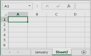
A workbook is a collection of worksheets. By default, a workbook has three sheets in Excel. You can delete or add more sheets to according to your requirements. By default, the sheets are named Sheet1, Sheet2 and so on .You can rename the sheet names to more meaningful names i.e. daily Expenses, Monthly Budget, etc.
Data Types:-
An Excel workbook file can hold any numbers of worksheets, and each worksheet is made up of more than 17 billion cells. A cell can hold any of three basic types of data:
- A numeric value
- Text
- A formula
A Worksheet can hold charts, diagrams, pictures, buttons and other objects.
Numeric Value:-Numeric values represent a quantity of some types such as, sales amounts, number of employees, number of students etc. Values can be dates or times such as (10:50a.m).
Numeric Limitations:-
Excel actually stores values with only 15 digits of precision. For example, if you enter a large value such as 123,456,789,123,456,789(18 digits).This 18-digit displays as 123,456,789,123,456,000.So it substitutes a zero for the last digits.
Text Entries:-
Most worksheets also include text in some of the cells. Text can serve as data (for example, a list of employee names), heading for columns or instruction about the worksheet.
Text that begins with a number is still considered text. For example, if you type 14 students into a cell, excel considered the entry to be text rather than a numeric value.
Formulas:-
Excel enables you to enter flexible formulas that use the values in cells to calculate a result. When you enter a formula into a cell, the formula’s result appears in the cell. Formulas can be simple mathematical expressions, or they can use some of the powerful functions that are built into excel.
Worksheet Basics:-
Every workbook contains at least one worksheet by default. When working with a large amount of data, you can create multiple worksheets to help organize your workbook and make it easier to find content. You can also group worksheets to quickly add information to multiple worksheets at the same time.
To rename a worksheet:
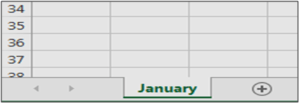
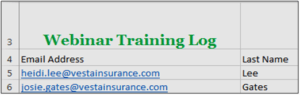
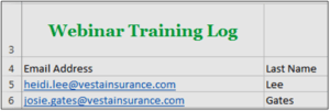
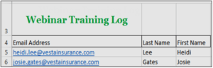
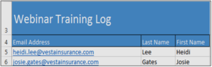
Whenever you create a new Excel workbook, it will contain one worksheet named Sheet1. You can rename a worksheet to better reflect its content. In our example, we will create a training log organized by month.
- Right-click the worksheet you want to rename, then select Rename from the worksheet menu.
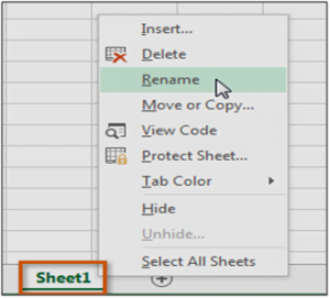
- Type the desired name for the worksheet.
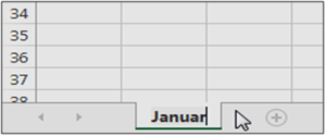
- Click anywhere outside of the worksheet, or press Enter on your keyboard. The worksheet will be renamed.
To insert a new worksheet:
- Locate and select the new sheet button.
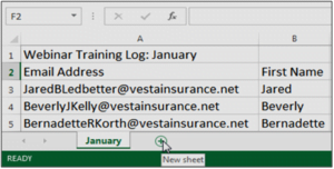
- A new blank worksheet will appear.
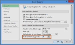
To change the default number of worksheets, navigate to backstage view, click Options, and then choose the desired number of worksheets to include in each new workbook.
To delete a worksheet:
- Right-click the worksheet you want to delete, then select Delete from the worksheet menu.
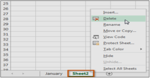
- The worksheet will be deleted from your workbook
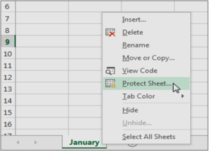
- If you want to prevent specific worksheets from being edited or deleted, you can protect them by right-clicking the desired worksheet and then selecting Protect sheet from the worksheet menu.
Understanding Cells and Ranges:-
A cell is a single element in a worksheet that can hold a value, some text, or a formula .A cell is identified by its address .For example, cell D5 is the cell in the fourth column and the fifth row.
A group of cell is called a range. A range in Excel is a collection of two or more cells.You designates a range address by specifying its upper –left cell and its lower right cell address, separated by colon (:). A cell range can be used inside a formula, for example to calculate the sum of the values within the selected cells: =SUM (A1:C6).
Range Example:-
- A range in Excel is a collection of two or more cells
Here are some examples of range addresses:-
| C24 | A range that consists of a single cell. |
| A1:B1 | Two cells that occupy one row and two columns. |
| A1:A90 | 90 Cells in a column A. |
Selecting Ranges:-
To perform an operation on a range of cells in a worksheet, first select the range .If you want to make the text bold for a range of cells, you must select range then choose Home Font Bold (Ctrl+B).
Deleting the contents of a cell:-
Delete the contents of a cell, just click the cell and press the delete key. To delete more than one cell, select all the cells that you want to delete and then press delete. Pressing delete removes the cells contents but doesn’t remove any formatting (such as bold, italic or different number format) that you may have applied to the cell.
You can choose Home Editing Clear. This command‘s drop-down list has five choices:-
Clear All:-Clears everything from the cell, its contents, its formatting.
Clear Formats:-Clears only the formatting and leaves, text, or formula.
Clear Contents:-Clears only the cells contents and leaves the formatting.
Clear Comments:-Clears the comments (if exists) attached to the cell.
Clear Hyperlinks:-Remove hyperlinks contained in the selected cells. The text remains, but the cell no cell no longer functions as a clickable hyperlink.
Home Tab
Text alignment:-
By default, any text entered into your worksheet will be aligned to the bottom-left of a cell, while any numbers will be aligned to the bottom-right. Changing the alignment of your cell content allows you to choose how the content is displayed in any cell, which can make your cell content easier to read.
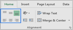
To change horizontal text alignment:
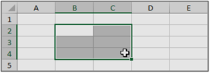
- Select the cell(s) you want to modify.
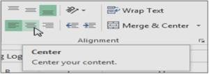
- Select one of the three horizontal alignment commands on the Home In our example, we’ll choose Center Align.
- The text will realign.
To change vertical text alignment:
- Select the cell(s) you want to modify.
- Select one of the three vertical alignment commands on the Home tab. In our example, we’ll choose Middle Align.
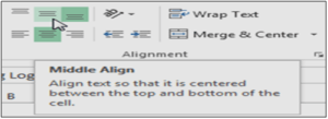
- The text will realign.
You can apply both vertical and horizontal alignment settings to any cell.
Cell borders and fill colors:-
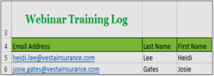
Cell borders and fill colors allow you to create clear and defined boundaries for different sections of your worksheet. Below, we’ll add cell borders and fill color to our header cells to help distinguish them from the rest of the worksheet.
To add a border:
- Select the cell(s) you want to modify.
- Click the drop-down arrow next to the Borders command on the Home tab. The Borders drop-down menu will appear.
- Select the border style you want to use. In our example, we will choose to display All Borders.
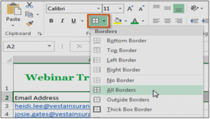
- The selected border style will appear.
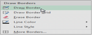
You can draw borders and change the line style and color of borders with the Draw Borders tools at the bottom of the Borders drop-down menu.
To add a fill color:
- Select the cell(s) you want to modify.
- Click the drop-down arrow next to the Fill Color command on the Home tab. The Fill Color menu will appear.
- Select the fill color you want to use. A live preview of the new fill color will appear as you hover the mouse over different options. In our example, we’ll choose Light Green.
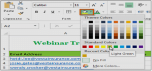
- The selected fill color will appear in the selected cells.
Instead of formatting cells manually, you can use Excel’s predesigned cell styles. Cell styles are a quick way to include professional formatting for different parts of your workbook, such as titles and headers.
To apply a cell style:
In our example, we’ll apply a new cell style to our existing title and header cells.
- Select the cell(s) you want to modify.
- Click the Cell Styles command on the Home tab, and then choose the desired style from the drop-down menu. In our example, we’ll choose Accent 1.
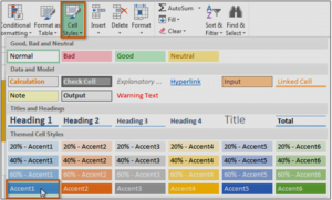
- The selected cell style will appear.
Applying a cell style will replace any existing cell formatting except for text alignment. You may not want to use cell styles if you’ve already added a lot of formatting to your workbook.
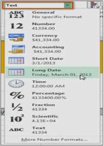
One of the most powerful tools in Excel is the ability to apply specific formatting for text and numbers. Instead of displaying all cell content in exactly the same way, you can use formatting to change the appearance of dates, times, decimals, percentages (%), currency ($), and much more.
Select the desired formatting option. In our example, we will change the formatting to Long Date.
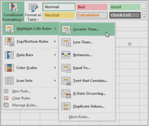
Conditional Formatting:-
Conditional formatting enables you to apply cell formatting selectively and automatically, based on the contents of the cells. For example, you can apply conditional in such a way that all negative values in a range have a light –yellow background color. Excel examines the value and checks the conditional formatting rules for the cell. If the value is negative, the background is shaded; otherwise, no formatting is applied.
Conditional formatting is an easy way to quickly identify cells of a particular type. You can use such as bright-red cells shading to make particular cells easy to identify.
If you have a worksheet with thousands of rows of data. It would be extremely difficult to see patterns and trends just from examining the raw information. Similar to charts and spark lines, conditional formatting provides another way to visualize data and make worksheets easier to understand.
To remove conditional formatting:
- Click the Conditional Formatting command. A drop-down menu will appear.
- Hover the mouse over Clear Rules, and choose which rules you want to clear. In our example, we’ll select Clear Rules from Entire Sheet to remove all conditional formatting from the worksheet.
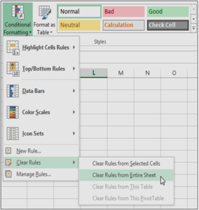
- The conditional formatting will be removed.
